Subcritical Coal-Fired Power Plant Flowsheet (steady state and dynamic)

Note

This is an example of a subcritical pulverized coal-fired power plant. This simulation model consists of a ~320 MW gross coal fired power plant, the dimensions and operating conditions used for this simulation do not represent any specific power plant. This model is for demonstration and tutorial purposes only.

Introduction

A 320 MW gross subcritical coal-fired power plant is modeled using the unit model library has been developed for demonstration purposes only. This plant simulation does not represent any power plant. This subcritical unit burns Illinois #6 high-volatile bituminous coal. The fuel is identical to the NETL baseline case for a 650 MW unit and its analysis data are listed in Table 1.

Table 1. coal specifications - Proximate Analysis (weight %)

item	As-Received	Dry
Moisture	11.12	0.00
Ash	9.70	10.91
Volatile Matter	34.99	39.37
Fixed Carbon	44.19	49.72
Total	100.00	100.0

Table 2. coal specifications - Ultimate Analysis (weight %)

item	As-Received	Dry
Moisture	11.12	0.00
Carbon	63.75	71.72
Hydrogen	4.50	5.06
Nitrogen	1.25	1.41
Chlorine	0.15	0.17
Sulfur	2.51	2.82
Ash	9.70	10.91
Oxygen	7.02	7.91
Total	100.00	100.0

Table 3. coal specifications - Heating Value

item	As-Received	Dry
Higher Heating Value (HHV), kJ/kg (Btu/lb)	27,113 (11,666)	30,506 (13,126)
Lower Heating Value (LHV), kJ/kg (Btu/lb)	26,151 (11,252)	29,544 (12,712)

The power plant is a generic subcritical unit, where the boiler has 4 levels of wall burners and one level of overfire airports. There are 18 platen superheaters hanging over the furnace roof serving as the finishing superheater. The platen superheater panels are parallel to the furnace side walls. The boiler has one drum, eight downcomers, backpass superheater, platen superheater, a reheater section (represented with 2 heat exchanger model), a primary superheater, an economizer, and the air preheater (this model is a simplified tri-sector Ljungström type)

The steam cycle equipment includes a multistage steam turbine with single reheat. It has a throttle valve, multiple stages for HP, IP, and LP sections with steam extraction to 3 low-pressure feed water heaters and 2 high-pressure feed water heaters as well as a deaerator and a boiler feed pump turbine. The steam cycle also includes the main and auxiliary condensers, a hotwell tank, a condensate pump, a booster pump and a main pump. Multiple control valves are used to control the water levels of hotwell tank, deaerator tank, and feed water heaters and the spray flow to main steam attemperator. The process flow diagram is shown in Figure 1. The entire process is modeled in two sub-flowsheets, one for the boiler system and the other for the steam cycle system, corresponding to two separate files named “boiler_subfs.py” and “steam_cycle_subfs.py”, respectively. The main flowsheet contains the two sub-flowsheets in a file named “plant_dyn.py”.

Figure 1: Process Flow Diagram

Property packages used:

• Helmholtz Equation of State (IAPWS95): Water and steam IAWPS95

• IDEAL GAS: Air and Flue Gas FlueGas

It can be seen from the Figure 1 that primary air is first split to two inlet streams, one goes through the primary air sector of the regenerative air preheater where it is heated, and the other, also known as tempering air, bypasses the air preheater and is used for primary air temperature control. The two streams are then mixed and connected with the fire side of the boiler. The coal stream is also fed to the fire side of the boiler. While this boiler sub-flowsheet does not contain a specific coal mill model, the partial vaporization of the moisture in the raw coal is modeled in the fire-side boiler model. The secondary air enters the secondary air sector of the air preheater. After being heated in the air preheater, the hot secondary air stream enters boiler’s windbox, from which it enters the furnace either as the secondary air of the burners or as overfire air. The pulverized coal from primary air stream is eventually burned in the boiler by both primary and secondary air to form flue gas that leaves the boiler with small amount of unburned fuel in fly ash. The hot flue gas then goes through the boiler backpass consisting of multiple convective heat exchangers including first the hot reheater, then the cold reheater, the primary superheater, and the economizer. Finally, the flue gas enters the air preheater to heat the cold primary air and secondary air before entering the downstream equipment which is not modeled. The feed water from steam cycle system enters the economizer to absorb the heat transferred from the flue gas and leaves the economizer at a temperature considerably below its saturation temperature. The subcooled water then goes to the boiler drum through water pipes where it mixes with the saturated water separated from the water/steam mixture from the boiler waterwall. The mixed water stream splits to two streams. A small amount of water leaves the system as a blowdown water to prevent buildup of slag and the main portion of the water stream goes through eight downcomers to enter the bottom of waterwall tubes. The vertical waterwall is modeled by multiple waterwall section models in series. The subcooled water from the downcomers is heated by the combustion products inside the boiler and part of the liquid are vaporized, forming a liquid-vapor 2-phase mixture and eventually enters the drum to complete a circuit for natural circulation of the feed water, in which the density difference between the liquid in the downcomers and the 2-phase mixture in the waterwall tubes drives the circulating flow.

The saturated steam from drum goes to the roof superheater before entering the primary superheater. Note that the enclosure wall tubes for the backpass as a part of the superheaters is not included in the flowsheet model. The steam leaving the primary superheater is mixed with spray water from boiler main feed pump in an attemperator. Finally, the steam from the attemperator enters the platen superheater where the steam is heated to main steam temperature before entering the main turbine. The cold reheat steam from the HP outlet is first heated in the cold reheater and then heated in the hot reheater before entering the IP stages of the turbine. There is no attemperation for the reheat steam.

The steam cycle, depicted in Figure 1, accepts steam from the boiler and uses it to generate electricity. Specifically, HP steam from the boiler passes through a throttle valve prior to entering the HP turbine, after which some is extracted to supply heat to feedwater heater (FWH) 6 while the remaining steam is sent back to the boiler to be reheated. The reheated steam then enters the IP turbine section where some is extracted to supply heat to FWH 5. Additional steam is extracted for the boiler feed pump turbine (BFPT) and deaerator between the IP and LP turbine sections at the IP/LP crossover, while the remaining steam enters the LP turbine. In the LP section, steam is extracted for FWHs 1, 2, and 3. Steam leaving the LP turbine is condensed in the main condenser, while steam leaving the BFPT is condensed in the auxiliary condenser. The condensate from the condenser hotwell is pumped through the LP FWHs 1, 2, and 3, where it is heated by steam extracted from the LP turbine. After passing through the deaerator, the feedwater enters a booster pump prior to entering the main boiler feed pump and HP FWHs 5 and 6.

Dynamic Flowsheet

The dynamic model considers the mass and energy inventories in large vessels in the system including drum, deaerator, feed water heaters, and condenser hotwell. Meanwhile, inventories in downcomers and multiple waterwall zones are also considered. To keep the problem tractable, the inventory in the 2D boiler heat exchanger model for the reheaters, the primary superheater, and the economizer are not considered. However, the internal energy held by the tube metal of those heat exchangers are considered. Some unit models are treated as the steady-state models on the dynamic flowsheet. For example, the boiler fire-side model is assumed as steady-state since the flue gas density is low and so is the residence time (2-3 seconds). All turbine stages, condensers and pumps are modeled as pseudo-steady-state. The entire process is pressure driven, indicating the flow rates of air, flue gas, water, and steam are related to the pressures in the system. Table 4 lists all unit operation models on the boiler sub-flowsheet including their names, descriptions, unit model library names, and dynamic/steady-state flag. Table 5 lists all unit operations on the steam cycle sub-flowsheet.

Table 4. List of unit models on the boiler system sub-flowsheet

Unit Name	Description	Unit Library Name	Dynamic
aBoiler	Boiler fire-side surrogate	BoilerFireside	False
aDrum	1D boiler drum	Drum1D	True
blowdown_split	Splitter for blowdown	HelmSplitter	False
aDowncomer	Downcomer	Downcomer	True
Waterwalls	12 waterwall zones	WaterwallSection	True
aRoof	Roof superheater	SteamHeater	False
aPlaten	Platen superheater	SteamHeater	False
aRH1	2D Cold reheater	HeatExchangerCrossFlow2D_Header HX2D	True *
aRH2	2D Hot reheater	HeatExchangerCrossFlow2D_Header HX2D	True *
aPSH	2D Primary superheater	HeatExchangerCrossFlow2D_Header HX2D	True *
aECON	2D Economizer	HeatExchangerCrossFlow2D_Header HX2D	True *
aPipe	Pipes from eco. to drum	WaterPipe	False
Mixer_PA	Mixer of hot PA and TA	Mixer	False
Attemp	Attemperator	HelmMixer	False
aAPH	Air preheater	HeatExchangerWith3Streams	False

• The heat held by tube metal is modeled as dynamic while fluids are modeled as steady-state

Table 5. List of unit models on the steam cycle system sub-flowsheet

Unit Name	Description	Unit Library Name	Dynamic
turb	Multistage turbine	HelmTurbineMultistage	False
bfp_turb_valve	BFPT regulating valve	HelmValve	False
bfp_turb	Front stage of BFPT	HelmTurbineStage	False
bfp_turb_os	Outlet stage of BFPT	HelmTurbineOutletStage	False
condenser	Main condenser	HelmNtuCondenser	False
aux_condenser	Auxiliary condenser	HelmNtuCondenser	False
condenser_hotwell	Mixer of 3 water streams	HelmMixer	False
makeup_valve	Makeup water valve	HelmValve	False
hotwell_tank	Hotwell tank	WaterTank	Dynamic
cond_pump	Condensate pump	HelmIsentropicCompressor	False
cond_valve	Condensate Valve	HelmValve	False
fwh1	Feed water heater 1	FWH0D	Dynamic
fwh1_drain_pump	Drain pump after FWH 1	HelmIsentropicCompressor	False
fwh1_drain_return	Mixer of drain and condensate	HelmMixer	False
fwh2	Feed water heater 2	FWH0D	Dynamic
fwh2_valve	Drain valve for FWH 2	HelmValve	False
fwh3	Feed water heater 3	FWH0D	Dynamic
Fwh3_valve	Drain valve for FWH 3	HelmValve	False
fwh4_deair	Mixer for deaerator	HelmMixer	False
da_tank	Deserator water tank	WaterTank	Dynamic
booster	Booster pump	HelmIsentropicCompressor	False
bfp	Main boiler feed pump	HelmIsentropicCompressor	False
split_attemp	Splitter for spray water	HelmSplitter	False
spray_valve	Control valve for water spray	HelmValve	False
Fwh5	Feed water heater 5	FWH0D	Dynamic
Fwh5_valve	Drain valve for FWH 5	HelmValve	False
Fwh6	Feed water heater 6	FWH0D	Dynamic
Fwh6_valve	Drain valve for FWH 6	HelmValve	False

• Dynamic flag is true for condensing section only

There are several control valves to regulate the water and steam flows in the steam cycle system including the throttle valve to control the power output, BFPT valve to control feed water pump speed and, therefore, the feed water flow, makeup water valve to control condenser hotwell tank level, condensate valve to control deaerator tank level, and water spray valve to control the main steam temperature. There are also drain valves between the drain outlet of a feed water heater and the drain inlet of its cascading downstream feed water heater. They are used to control the water level inside the condensing section of the feed water heater.

Controllers are included in the dynamic flowsheet. There are several regulatory level controllers, all of which are either PID controllers, including those to control the levels of FWH2, FWH3, FWH5, FWH6, deaerator tank, and hotwell tank. The corresponding control valves involved in those level controllers are drain valves of FWH2, FWH3, FWH5, FWH6, the condensate valve, and the makeup water valve, respectively.

The main steam temperature is controlled by the attemperator with the spray water from the main feed pump outlet. The spray valve between the attemperator and the feed pump outlet is controlled by a PID controller that is also configured with default valve opening bounded between 0.05 and 1. This configuration limits the spray flow to certain values if the main steam temperature is way below or above its setpoint.

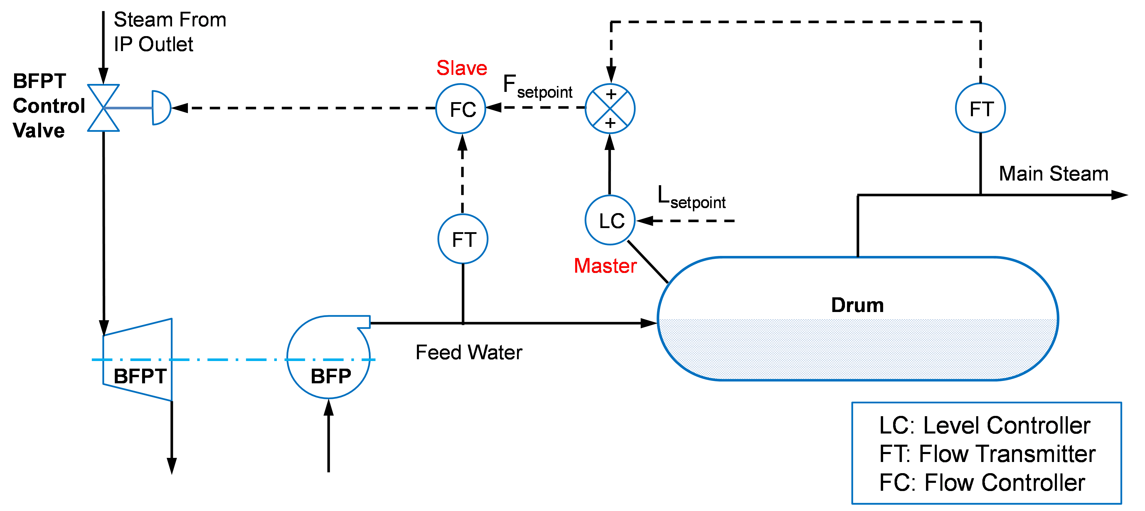
The drum level is controlled by a 3-element controller as shown in Figure 2. It is implemented with two cascading PI control loops. The master controller of the drum level cascading control is used to provide the setpoint of the slave controller. The slave controller controls the feed water flow rate based on the setpoint provided by the master controller. The three measured elements include drum level, main steam flow and feed water flow. Note that the main steam flow rate is usually controlled by a throttle valve such that the required power output is met. The feed water flow rate should be the same as the main steam flow rate in a steady-state condition. If the drum level is deviated from its setpoint, the feed water flow should be adjusted to compensate the level deviation. For example, when the drum level is too low, the feed water flow rate should be increased. Therefore, the setpoint of the feed water flow rate for the slave controller is equal to the sum of the measured main steam flow rate and the output of the master controller, which is the adjustment calculated by the master controller due to the deviation of the drum level from its setpoint. In case there is a drum water blowdown flow, the amount of blowdown flow should also be added. In the modeled power plant, the flow rate of feed water is controlled by the governing valve of the boiler feed pump turbine (BFPT), which controls the speed of the BFPT and hence the speed of the boiler feed pump (BFP). The BFPT uses the steam from the IP turbine outlet to generate the mechanical work needed for the BFP pump.

Figure 2: Drum Level Control

The supervisory level control for the power generation is implemented as a typical coordinated control as shown in Figure 3. It involves a turbine master that controls the throttle valve opening to meet the power demand and a boiler master that controls the coal feed rate and air flow rates. In the dynamic flowsheet model, both the turbine master and the boiler master are implemented as PI controllers. The turbine master simply controls the power output to meet the power demand by adjusting the throttle valve opening. The boiler master controls the coal feed rate and air flow rates to maintain the desired main steam pressure. The setpoint for the main steam pressure is calculated as the sum of two parts. The first part is the desired steady-state sliding pressure as a function of load (sliding pressure curve as shown in the figure). In the current dynamic plant model, the sliding pressure is implemented as a linear function of power demand. The second part is the pressure adjustment term calculated based on the deviation of electrical power output from the demand multiplied by a gain factor. The second part represents the coordination between the turbine master and boiler master. Note that in the current dynamic flowsheet model, the control for the air flows is not implemented with detailed PID controllers for FD and ID fans and their dampers. The primary and secondary air flow rates are actually specified as constraints such that the mole fraction of O2 in flue gas is set to be a predefined function of coal flow rate, which is related to the load. The primary air flow rate is specified as a constraint that specifies the primary air to coal flow ratio as a function of coal feed rate (mill curve). In other words, the primary and secondary air flow rates is controlled in proportion to the coal feed rate as in a typical ratio control loop.

Figure 3: Coordinated Control

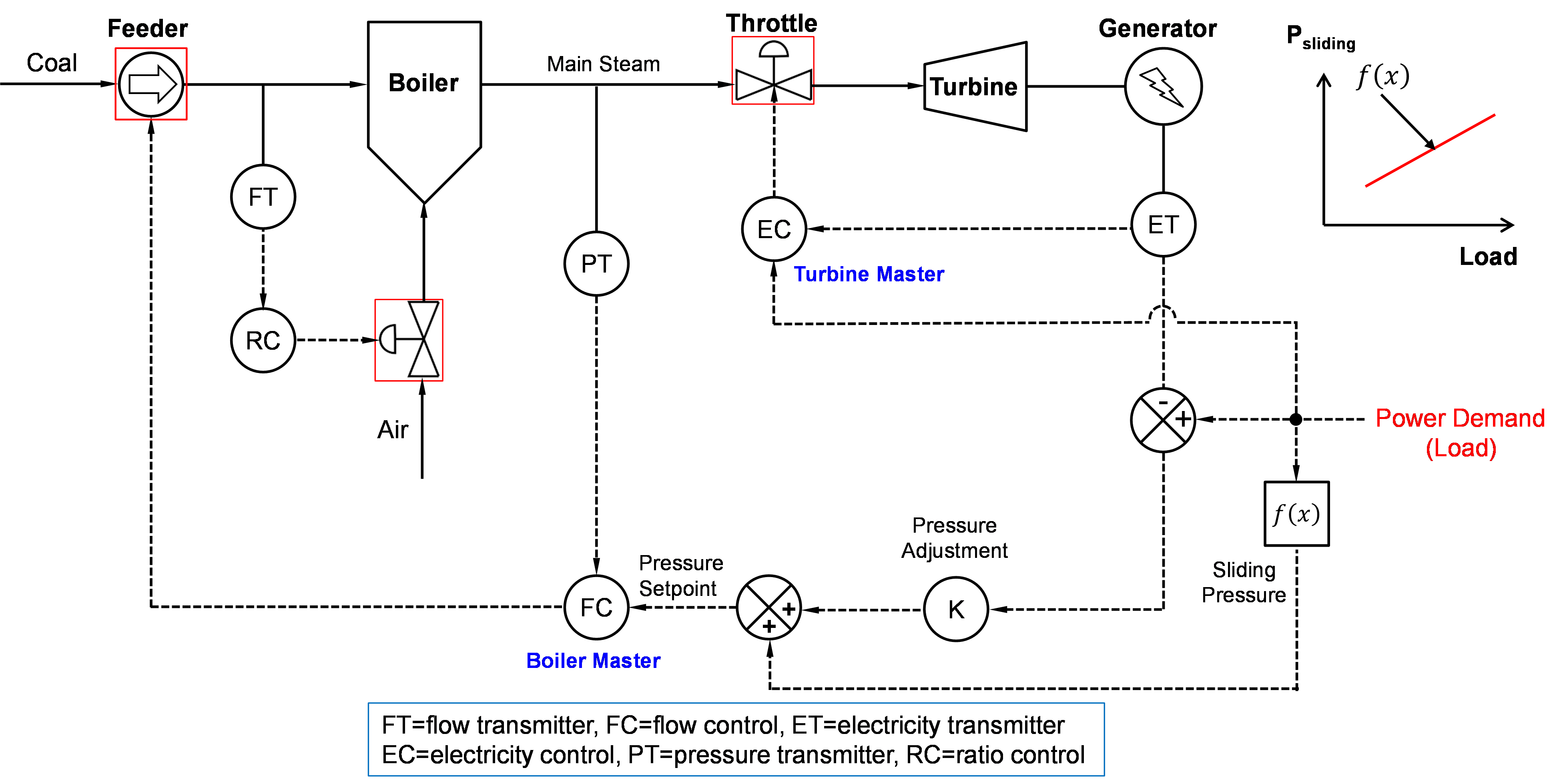
Table 6 lists the PI and PID controllers on the dynamic flowsheet. Some controllers are declared on the steam cycle sub-flowsheet while others are declared on the main flowsheet. The table also lists the type of the controller, whether it is bounded for output, and whether it belongs to the steam cycle or main flowsheet.

Table 6. Controllers in the dynamic flowsheet model

Unit Name	Description	Type	Bounded	Flowsheet
fwh2_ctrl	Level controller for FWH 2	PI	No	Steam cycle
Fwh3_ctrl	Level controller for FWH 3	PI	No	Steam cycle
Fwh5_ctrl	Level controller for FWH 5	PI	No	Steam cycle
Fwh6_ctrl	Level controller for FWH 6	PI	No	Steam cycle
da_ctrl	Level controller for deaerator tank	PI	No	Steam cycle
makeup_ctrl	Level controller for hotwell tank	PI	Yes	Steam cycle
spray	Main steam temperature controller	PID	Yes	Steam Cycle
drum_master_ctrl	Master controller for drum level	PI	No	Main
drum_slave_ctrl	Slave controller for drum level	PI	No	Main
turbine_master_ctrl	Turbine master controller	PI	No	Main
boiler_master_ctrl	Boiler master controller	PI	No	Main

Steady-state power plant example:

A steady state version of the power plant flowsheet is constructed by calling the m_ss = main_steady_state() method line 1824 in the subcritical_power_plant.py file. This function will build a steady state version of the power plant in Figure 1. This power plant model consists of two subflowsheets, the boiler subsystem (m_ss.fs_main.fs_blr) and the steam cycle subsystem (m_ss.fs_main.fs_stc. These two subsystems are connected trough arcs at the flowsheet level. A custom initialization procedure has been developed, in which we initialize each subflowsheet at the time at a given load. After initializing the subflowsheet the example solves the entire power plant model for a given load (degrees of freedom = 0).

Main Fixed Variables:

• power demand (m_ss.fs_main.power_output.fix(320))

• main steam temperature (m.fs_main.fs_stc.temperature_main_steam.fix(810) in Kelvin)

• water level (drum, deareator, condenser, feedwater heaters)

• equipment geometry/dimension

• fuel composition and HHV (on dry basis)

Main unfixed variables calculated by the model: * Coal flowrate (m.fs_main.fs_blr.aBoiler.flowrate_coal_raw is unfixed and calculated to match the power demand) * water/steam flowrates * attemperator flowrate (m.fs_main.fs_stc.spray_valve.valve_opening.unfix()) free to keep main steam at 810 K * Boiler feedwater pump pressure (m.fs_main.fs_stc.bfp.outlet.pressure.unfix()) * throttle valve opening (m.fs_main.fs_stc.turb.throttle_valve[1].valve_opening.unfix()) * primary air and secondary air flowrates (constrained by primary air to coal ratio and O2 mol fraction in the flue gas)

Dynamic power plant example:

The dynamic simulation version of the power plant examples is built when the user calls the m_dyn = main_dynamic() method in line 1820 in the subcritical_power_plant.py file. The user should note that this method takes a long time to solve (~60 min). This method builds and runs a subcritical coal-fired power plant dynamic simulation. The demonstration example prepared for this simulation consists of 5%/min ramping down from full load to 50% load, holding for 30 minutes and then ramping up to 100% load and holding for 20 minutes.

This method first creates a steady state version of the power plant, initializes the steady state model, and then uses this steady state model for initializing the dynamic model. Two dynamic flowsheets are constructed here, the main difference is that they have different time steps in the discretization domain. Dynamic flowsheet 1 uses a step size of 30 seconds and dynamic flowsheet 2 uses a time step of 60 seconds. This is useful to speed up the overall simulation time and to reduce the final number of variables and constraints. Note that the dynamic flowsheet 1 is used when the load is changing to capture the dynamic transient conditions of the plant change (i.e., while plant is ramping). While the dynamic flowsheet 2 is used when process is near steady state transient conditions. To simulate the dynamic case, this example implements a ramp function for the power demand and fixes the set point to match the power demand (see code below).

for t in m.fs_main.config.time:
    power_demand = input_profile(t0+t, x0)
    m.fs_main.turbine_master_ctrl.setpoint[t].value = power_demand

Solving the dynamic model:

At this point we have a very large mathematical model, therefore, to exploit the temporal distribution of the model. The team implemented a rolling horizon approach (also known as receding horizon or moving time window), in which the full space model is divided into subproblems with 2 time periods each, then we solve the subproblem and use the solution of the previous subproblem to connect with the next time window (each time window consists of a dynamic model with 2 time periods). Thus, the dynamic model with 2 time steps is solved based on the disturbance of load demand specified by the user (power demand function described above). If the time duration for the simulation is longer than the period of the 2 time steps, the results of the solved dynamic model at the end of the second time step will be copied as the initial condition for the simulation of the next 2 time steps. The results to be copied include the errors for the integral and derivative parts of individual controllers. In case the error term for the integral part of a controller is too large (windup error), the user has an option to reset the windup error. If the time step size is changed, the user needs to choose a different dynamic model to copy to (dynamic flowsheet 1 or dynamic flowsheet 2). After that the time window is rolled to the second one and the simulation for the second time period can then be solved. This process is repeated for multiple time periods until the entire duration for the dynamic simulation is solved.

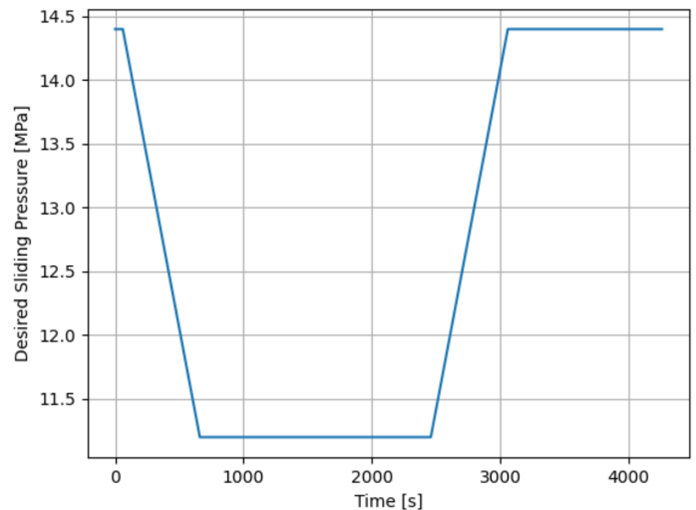
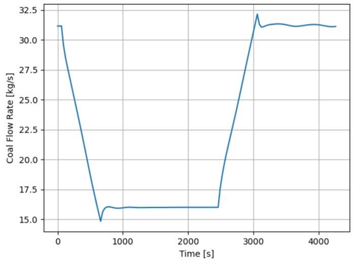
Note that during each rolling time window simulation, the results at individual time step for the main performance variables and equipment health are saved. Those results are plotted after the last simulation and written to a text file for review and further processing. Figure 4 shows an example of dynamic model simulation result, the load demand (ramp function) and coal feed rate for as functions of time.

Figure 4: Transient results for a load changing dynamic simulation